Moving Forward with
Magnitude-Based Decisions: recent progress
Will G Hopkins, Institute for Health and Sport, Victoria
University, Melbourne, Australia. Email. Update Dec 2020. The Lohse et al.
review of MBI mentioned in this item, and which appeared first in the SportRxiv, was published in PLoS
One in August (Lohse et
al., 2020b). Also published there is a critique in which
Janet Aisbett (2020) identifies major flaws in
the data and conclusions of the review. Follow this link to the SportExSci mailing list
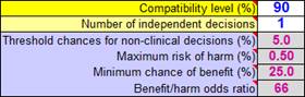
for a summary and links. In this In-brief item I summarize recent developments with magnitude-based decisions (MBD), including an introduction to the article in the current issue on the topic of MBD expressed as hypothesis tests (Hopkins, 2020). I have tried to make that article accessible to non-statisticians, but it is a long hard read, so I also present here a shorter, plainer language description of MBD, by showing its similarity to null-hypothesis significance testing. See also an updated version of a slideshow first presented at the German Sport University last July. At the end of this item, I explain important updates to some of the spreadsheets at this site, including extra advice on choosing smallest importants for MBD. As a visitor to this site, you probably know that magnitude-based inference (MBI) is a method for making conclusions in studies of samples, taking into account the fact that a sample gives only an approximate estimate of the true (very large sample) value of an effect. Even if you don't really understand MBI, you almost certainly know that MBI has been criticized by Kristin Sainani and others for lack of a theoretical basis and for high error rates (Sainani, 2018; Sainani et al., 2019), resulting in some journals banning MBI. I contacted the statistician Sander Greenland over a year ago for help with addressing these criticisms. I was then able to show that MBI does have a theoretical basis in Bayesian statistics, to the extent that the probabilistic assertions in MBI about the magnitude of the true effect (possibly beneficial, very likely increased, likely trivial, and so on) are practically the same as those from a semi-Bayesian analysis with a realistic, proper, weakly informative prior (Hopkins, 2019a, 2019b; Mengersen et al., 2016). Alan Batterham and I had already shown that the error rates, defined as making wrong conclusions about substantial and trivial magnitudes, were generally lower than with null-hypothesis significance testing, and often much lower (Hopkins & Batterham, 2016). Greenland nevertheless suggested that the decision process in MBI should be formulated as hypothesis tests, since some error rates would be transparently well-defined by such tests, and statisticians of the traditional frequentist persuasion would then be more likely to accept MBI as a useful tool. He also suggested removing inference from the name of the method, because he believes that this word should be reserved for making conclusions that take into account not just sampling uncertainty but all the uncertainties in a study, including representativeness of the sample, validity of the measures, and accuracy of the statistical model used to estimate the magnitude of the effect. I therefore opted to rename MBI as magnitude-based decisions (Hopkins, 2019a), and I contacted Alan Batterham and psychologist-statistician Daniel Lakens for help with the hypothesis tests that underlie MBD. By July last year I had finished a first draft of the accompanying article, when Alan and I were contacted out of the blue by a retired mathematics professor named Janet Aisbett. She had independently shown that MBD is equivalent to several hypothesis tests and had also written a first draft of an article intended for a statistical journal. Janet next contacted Sander Greenland for feedback, and as a result he, Janet, Daniel, Alan, Kristin and I have been exchanging emails in a futile attempt to reach a consensus about MBD. The article submitted by Aisbett et al. (2020) includes recommendations to drop the Bayesian interpretation, drop multiple alpha levels, and drop the MBD method of sample-size estimation. I can't agree with these recommendations. I also think that MBD should be presented in a deservedly more positive way, as a valuable inferential tool. There is agreement on the big picture, that MBD is equivalent to several hypothesis tests about substantial and trivial magnitudes. The tests define acceptable Type-2 (false-negative or failed-discovery) error rates, regardless of sample size. The Type-1 (false-positive or false discovery) error rates are not controlled, and in the clinical version of MBD they are sometimes higher and often lower than those of classic null-hypothesis significance testing (NHST), depending on sample size and true effect. But the effects are presented with probabilistic terms that properly reflect the level of evidence for benefit. Rejection of at least one hypothesis represents a publishable quantum of evidence about the magnitude of an effect, and there is no substantial publication bias with the sometimes unavoidably small sample sizes in sport research. In short, MBD has a valid frequentist basis and provides an avenue for researchers to publish such studies without compromising the literature. In fact, MBD benefits the literature, because those studies can contribute to meta-analyses. The way MBD works is similar to that of NHST, but an improvement in several respects. NHST is all about testing to see if the true effect could be null or zero. You get a probability (p) value for that test, and if the p value is low enough (usually <0.05), you reject the hypothesis that the effect is null; you thereby decide that the effect is not null, and you say the effect is statistically significant. MBD, in contrast, is all about testing to see if the effect could be substantial rather than null. Rejection of the hypothesis that the effect is substantial of a given sign results in the decision that the effect is not substantial of that sign, and you say the effect is clear rather than significant (but see the end of this item for advice when applying clear to magnitudes rather than effects). Importantly, the p value for the test of a substantial magnitude is the same as the MBD chances (expressed as a probability) that the true effect is substantial: beneficial or harmful for clinically or practically important effects resulting in consideration for implementation of a treatment, or substantially positive or negative for non-clinical effects, such as a mean difference between males and females. The p-value threshold is 0.005 for the hypothesis of harm, 0.25 for the hypothesis of benefit, and 0.05 each for the hypotheses of substantial positive and negative. Notice that NHST has only one hypothesis to test, whereas MBD has two. In NHST, failure to reject the null hypothesis results in declaration of a statistically non-significant effect. In MBD, failure to reject both hypotheses (harm and benefit, or substantially positive and negative) results in declaration of an unclear effect, which is another way of saying the effect could be beneficial and harmful (or substantially positive and negative), that precision is therefore inadequate or that uncertainty is unacceptable, and that the finding is indecisive or inconclusive and therefore potentially not publishable. Herein lies an important difference between NHST and MBD. When you get non-significance in NHST, it seems natural to conclude that the effect is unimportant or trivial, but such a conclusion is justified only when the sample size is greater than or equal to the sample size estimated for the chosen power of the study (usually 80%, meaning you would have an 80% chance of getting statistical significance if the effect is the smallest important substantial value). Similarly, if you get significance, it seems natural to accept the underlying alternative hypothesis and conclude that the effect is important, but such a conclusion is justified only when the sample size is less than or equal to the estimated sample size. If you get significance with a large sample size or non-significance with a small sample size, or if you aren't sure whether your sample size is large or small, it's easy to make an unjustified conclusion, so misinterpretations of outcomes using NHST are widespread. For this and other reasons, Greenland and co-authors have called for the retirement of statistical significance (Amrhein et al., 2019). I believe that MBD is a worthy successor to NHST. When you get an unclear outcome, you know that you need more data–in fact, the spreadsheets at Sportscience tell you to get more. There is no such overt or implied advice with NHST, unless you deem all non-significant effects to be unclear, in what Alan and I called conservative NHST (Hopkins & Batterham, 2016). When you get a potentially publishable outcome in MBD as a result of rejecting one hypothesis, the test of the other hypothesis provides additional probabilistic information about the magnitude of the effect: the p value for that test is the same as the MBD chances (expressed as a probability) that the true effect has that substantial magnitude. There is no such overt or implied information in NHST. And rejection of both hypotheses with p<0.05 (very unlikely substantial) implies that the true effect is decisively trivial. The decisions in MBD are also not dependent on a pre-set sample size: the smaller the sample size, the more the uncertainty, of course, but the uncertainty is up front in plain language, whereas NHST offers only significance and non-significance. In this respect, MBD gives particularly realistic outcomes when the true effect is close to the smallest important threshold; for such effects, there is a sense in which the correct decision is that the effect could be trivial or substantial (as shown by a simple consideration of the coverage of the compatibility interval, even for narrow intervals arising from large sample sizes), and this is the decision that MBD delivers most of the time. It is only when the interval falls entirely on the side of the smallest important away from the true effect that mistakes are made, at most ~5% of the time with a 90% interval. A point of contention is sample-size estimation. In MBD, sample size is determined by marginal rejection of both substantial hypotheses, thus avoiding an unclear outcome, whatever the true effect. Aisbett et al. (2020) would instead prefer sample size to be large enough to show either that an effect is decisively substantial (via minimal-effects testing, MET) or that it is decisively trivial (via equivalence testing, ET). The problem with both these approaches is that true effects close to the smallest important require unrealistically large sample sizes to deliver rejection of the relevant hypothesis (non-substantially +ive or –ive for MET, non-trivial for ET). The researcher therefore has to posit that the true effect is "expected" to be a value somewhat larger than the smallest important (for MET) or somewhat smaller than the smallest important (for ET) in the hope of an achievable sample size. As I show in the accompanying article, the MBD sample size is consistent with that of MET for a modest expected substantial effect (marginal small-moderate), but the sample size for ET is unrealistically large for any reasonable expected trivial effect. In any case, I am not convinced by the rationale for "expected" effects. I therefore see no reason to modify the method of sample-size estimation in MBD, but researchers should be aware that it is a minimum desirable sample size. I regret calling it previously an optimum sample size. The fact that this sample size is approximately one-third that required for 80% power and 5% significance in NHST does not in itself imply that MBD promotes studies with samples that are too small. I have never recommended anything less than the minimum desirable sample size, but researchers who can't reach the minimum will still get a trivially biased, useful and potentially publishable outcome, if one hypothesis is rejected. Larger sample sizes are always more desirable to reduce the uncertainty in the magnitude, especially when researchers want to quantify the modifying effects of subject characteristics, mediators representing potential mechanisms of the effect, and standard deviations representing individual responses. Larger sample sizes and stricter decision criteria are also required to constrain overall error rates with more than one effect in a study. Another point of contention is the probabilistic terms describing the magnitude. In MBD, once one hypothesis has been rejected (e.g., harm), the p value for the other hypothesis test (benefit) is the reference-Bayesian probability that the effect has that other magnitude, when the prior is practically uninformative. The probabilities are given the interpretation of possibly, likely, very likely and most likely for p>0.25, p>0.75, p>0.95 and p>0.995 respectively. Aisbett et al. (2020) have suggested strictly frequentist interpretations of these p values: the effect (the data and model) is ambiguously, weakly, moderately and strongly compatible with that substantial magnitude. So it's a question of whether possibly beneficial underestimates the uncertainty, where ambiguously compatible with benefit does not. Or does ambiguously compatible actually overestimate the uncertainty or even confuse the practitioner? Possibly beneficial may send a more accessible message to practitioners about the potential implementability of a treatment, assuming of course that harm was most unlikely (strong rejection of the hypothesis of harm), but it is important for everyone to be aware of the assumptions that the model is accurate, the measures are valid, and the sample is representative of the population. It is also important with small sample sizes to check whether a weakly informative prior modifies the probabilities and the magnitude-based decision (Hopkins, 2019b); if it does, or if a more informative prior is justified, the modified decision should be presented. Furthermore, the possibility of individual responses to a treatment should be acknowledged and taken into account with appropriate error terms and subject characteristics as effect modifiers. I am convinced that the reference-Bayesian interpretation of outcomes in MBD is valid, accessible and useful. I have therefore replaced Bayesian with frequentist terms in only one spreadsheet, the one that converts an NHST p value to MBD. A link to the original version is available in the spreadsheet. See also the appendix in the MBD article in this issue for advice on reporting MBD in manuscripts for journals requiring emphasis on hypothesis tests. The spreadsheets for analyzing crossovers, controlled trials, and group means now contain an explanation of the decision process in terms of hypothesis tests, as comments in the left-hand cells of this panel (with 90 inserted; that cell is blank in the spreadsheets):
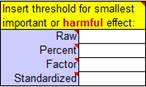
You can make the "alpha" levels (p-value thresholds for the hypothesis tests, shown as percents in the above cells) more conservative in a systematic manner by choosing a 95% or 99% compatibility level or by increasing the number of independent decisions to 2 or more. You can also change the alpha levels individually. Janet Aisbett also detected in the spreadsheets inconsistent handling of clear effects that were possibly trivial and possibly substantial. All the spreadsheets now show such effects as possibly substantial, but that needn't stop you from presenting such effects as possibly trivial and possibly substantial to emphasize the uncertainty, as shown in the Bayesian section of the Appendix of the accompanying article. An appropriate value of the smallest important effect is crucial for making a magnitude-based decision. One option is standardization, in which a difference or change in means is divided by an appropriate between-subject standard deviation to get Cohen's d (with a smallest important of ±0.20). Researchers appear to have been using standardization as a default (Lohse et al., 2020), whereas it is better as a fallback, when there is no way to quantify the relationship between the effect and health, wealth or performance. I have updated the comments in this panel of the spreadsheets to emphasize this point:
For more on magnitude thresholds, see the slideshows linked to the article on linear models and effect magnitudes (Hopkins, 2010). Finally, MBI has been criticized for its misuse by some researchers, who have applied non-clinical MBI to clinically important effects (presumably to get a publishable outcome when the clinical decision was unclear), or who have dropped the terms possibly, likely and so on from the description of the effect, making the magnitude seem definitive (Lohse et al., 2020; Sainani et al., 2019). Such misuse can be reduced with more vigilance by researchers, reviewers and editors. The term clear can also take some blame, because researchers may think that a clear effect with an observed substantial (or trivial) magnitude is the same as a clearly substantial (or trivial) magnitude. Again, inclusion of the probabilistic term prevents any mistake: a clear possibly substantial effect is obviously not clearly substantial. The terms clearly, decisively or conclusively can and should be applied to a magnitude, but only when it is very likely or most likely substantial or trivial (the effect is moderately or strongly compatible with the magnitude, to use the frequentist terminology). For references, see below. When N is <10: how to cope with very small samplesWill G Hopkins,
Institute for Health and Sport, Victoria University, Melbourne, Australia. Email. A sport scientist recently emailed me for advice on how best to investigate the effect of a treatment when the sample is the national team of only six athletes. See below for my response. In summary, the problem with small sample sizes is usually inadequate precision for the mean effect of the treatment. You can improve precision to some extent by testing each subject multiple times pre and post the treatment or, where possible, by administering the treatment to each subject multiple times. The extra data for each subject may also allow a decision about each individual’s response to the treatment. Please note that my advice does not represent endorsement of studies with small sample sizes. You study a sample to get an estimate of the mean effect not just in the sample but in the population represented by the sample. In other words, you would like the mean effect in the sample to be the mean effect with any and all subjects similar to the sample. But the mean effect in a small sample may differ substantially from the mean in the population, for two reasons. First, if you measured the same subjects again pre and post the treatment, you would get a different answer arising from random error of measurement. Secondly, if there are individual responses to the treatment, a small sample can easily have a distribution of responses different from that in the population. The compatibility (formerly confidence) interval for the mean effect properly accounts for these two sources of sampling variation, but with a small sample you may get a compatibility interval so wide that the mean effect of the treatment is indecisive. The spreadsheets at Sportscience tell you: unclear, get more data. You can get more data by testing each subject several times and averaging the measurements pre and post the treatment. The error in the average of n measurements is the error in any one measurement reduced by a factor of 1/Ön, and if there are n measurements pre and n measurements post the treatment, the width of the compatibility interval is reduced by a factor of at most 1/Ön. I say at most, because the time between pre and post measurements is inevitably longer than the time required to administer each of the two clusters of multiple measurements, so additional error of measurement may creep in between pre and post. For example, you could administer several performance tests over a period of a week and average them, but if the treatment is some kind of training that takes months to administer, there is likely to be additional error that is not reduced by the averaging. Individual responses to the treatment also manifest as additional error between pre and post. The only way to get around the problem of this extra error is to re-administer the treatment and the pre- and post-tests after a period sufficient to wash out the effect of the treatment. (For a training treatment, the wash-out period might need to be the off-season.) You then average the effect of the multiple administrations in each subject, then analyze the averages, or better still, use mixed modeling to deal with the multiple clusters of measurements. A mixed model will also deal properly with a sample consisting of participants with different numbers of repeated measurements, for example when you repeat the treatment in consecutive seasons on a team whose composition changes, or when the treatment and time combinations differ between participants (e.g., Vandenbogaerde & Hopkins, 2010). Whether you use one of my spreadsheets or a mixed model to do the analysis, keep in mind that excessive uncertainty arising from a small sample size can make unrealistic probabilities of substantial and trivial magnitudes for a magnitude-based decision. You should therefore do a Bayesian analysis to check whether a weakly informative prior "shrinks" the magnitude and its compatibility limits, and if it does, present the original and Bayesian-modified effect and probabilistic decision. Read this article (Hopkins, 2019b) for more, and use this spreadsheet (the Bayes tab) to do the Bayesian analysis. A spin-off of multiple measurements is the possibility of estimating the effect with enough precision to determine each individual’s response to the treatment. Presenting your study to a journal as a case series, with each individual analyzed separately, might also go down better with reviewers than an analysis of a sample with an embarrassingly small sample size. Error of measurement needs to be preferably less than half the smallest important change to make individual assessments with a single pre- and post-test, as you can see for yourself by playing with the spreadsheet for assessing an individual (the first tab) (Hopkins, 2017). Unfortunately, errors of measurement of athletic performance tests are often several times greater than the smallest important change in performance. For example, if the test measure is competitive performance time or distance itself, or is highly correlated with it, the smallest important is 0.3x the error of measurement, so the error is 1/0.3 = 3.3x the smallest important (Hopkins et al., 2009), so you will need many measurements pre and post a treatment to reduce the error. How many? The analysis is effectively the same as when you compare the means of two groups of subjects, with the two groups being the pre and post measurements. The sample-size spreadsheet (Hopkins, 2006) shows 120 measurements: 60 pre and 60 post! With only a few repeated measurements, trivial or small observed mean changes in the individual athlete would be inconclusive. So if you want to monitor performance of an individual, you have to find a performance test that has a smaller error than competitive performance itself, and the athlete and coach will have to be happy for the test to be done well at least weekly. The spreadsheet for assessing an individual includes a tab for monitoring an individual with regular testing. If you are doing an intervention with an athlete, the spreadsheet effectively averages multiple pretests by fitting a trend line. Test scores during or after an intervention are assessed relative to the extrapolated trend line, and you can average such tests to improve the precision. Read the article accompanying the spreadsheet (Hopkins, 2017) for more. Having monitored six or so athletes with reasonable precision, the outcome could be several showing reasonable evidence of benefit, several showing some evidence of harm, and the others showing an unclear effect (or, less likely, a clearly trivial effect). What kind of conclusion could you then make about the effect of the treatment on other athletes? The safest conclusion is that there are probably individual positive and negative responders, and that the treatment should therefore not be administered to the whole team. A much larger sample and appropriate analysis would be required to identify the characteristics of positive responders that would allow them to be targeted with the treatment. SAS Studio Changing to Online Access OnlyWill G Hopkins,
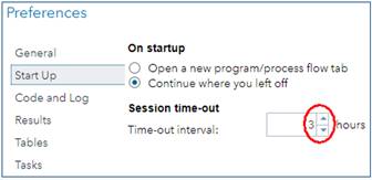
Institute for Health and Sport, Victoria University, Melbourne, Australia. Email. SAS Studio University Edition (Studio UE) is the SAS Institute's answer to the free statistics package, R Studio. SAS does some aspects of data processing and all aspects of mixed modeling better than R, and SAS's programming language is more user-friendly, so I have promoted Studio UE with a suite of self-paced learning materials. If you are already a user of Studio UE, you will have received an email from SAS in November about its replacement by a version of SAS Studio running in the cloud and accessed via On Demand for Academics (Studio ODA). Studio UE will not be available after July 2021. I have now made the transition, and this In-brief item represents my report on Studio ODA, followed by my advice on getting started. First, the good news about Studio ODA... • It is still free. • It runs faster (by 25% compared with my fast laptop, although it may depend on how many other people are using it online). • If you are a first-time user, you won't have the considerable challenge of installing a virtual server to run SAS Studio on your laptop. Ignore the info about installing a server and SAS Studio in my suite of materials. • You won't have to install updates. But there's some bad news... • You now have to be online to use SAS (obviously), so forget about running programs, if your net connection is down or you're on a long-haul flight. (Emirates has wifi on many routes, but the bandwidth for anything other than email is hopeless.) • You cannot run programs stored on your laptop directly from your laptop, which means you have to upload them and any data files into the Server Files and Folders window of the online version. • You cannot upload directories, so you have to create a directory structure in the Server Files and Folders window, directory by directory. • If you want to share programs with anyone, or save them for offline use, you have to download them, one file at a time. There is no facility for synchronizing files between your laptop and the SAS server. However, Results files can be downloaded directly to your laptop, and there is an email icon for sending Results and/or the program that produced them to anyone. • You are logged out automatically after a certain period of inactivity (default = 1 h), but the most you can set the period to is only 3 h. Set it to 3 h when you first use Studio ODA, via the Preferences/Start-Up menu:
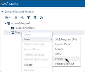
• You are logged out automatically after six hours, so you can't run complex mixed models with large datasets that previously took overnight to run. And now here's my guide to making the transition. The email from SAS includes this getting started link. Click on it and you will get a browser window with four steps to follow. SAS UE users, who already have a SAS profile, can skip Step 1. The next three steps are easy, and by the time you finish, you will have opened a window in a browser that looks almost exactly like Studio UE. The only difference is a practically empty Server Files and Folders frame at the top left. You have to populate that frame with your folders and files. Unfortunately you have to do it one folder at a time. The instructions on the getting-started page (under this drop-down: Uploading data and programs into ODA) tell you how to upload files, but there's nothing there about creating folders. Do it by right-clicking on the Files (Home) icon and selecting New/Folder:
After naming the folder, right-click on it to create a folder within a folder. I suggest you recreate your folder structure exactly as you already have it on your laptop. You can then right-click on a folder and select Upload Files... If you end up with many folders within folders, you can create shortcuts to the ones you use a lot by right-clicking on Folder Shortcuts, but I suggest you leave that until later or not even bother with it. Once you have uploaded a program and any data that it needs, run it in Studio ODA exactly as you do in Studio UE, but you will first have to change all the FILENAME and LIBNAME statements. Simply delete everything in front of the name of the top-most folder. For example, in Studio UE, I had this: FILENAME REFFILE '/folders/myshortcuts/VU Melbourne/John Smith/Erg validity/ erg data.xls'; In Studio ODA, I deleted /folders/myshortcuts/ to get
this: Another option is available on the Getting Started page, under the instructions for Modifying your LIBNAME statement so it works on ODA (they forgot to mention FILENAME statements). For example, you end up with this, which also works: FILENAME REFFILE '~/VU Melbourne/John Smith/Erg validity/erg data.xlsx'; If you make a mistake with a FILENAME or LIBNAME statement, double-click on an Excel spreadsheet in the same folder and check the CODE window to see the FILENAME that SAS assigns. I got this with the above spreadsheet: FILENAME REFFILE '/home/will17/VU Melbourne/ John Smith/Erg
validity/erg data.xlsx'; You will see your SAS profile name instead of mine (will17). Copy the text between quotes with or without the Excel filename, and paste it into your FILENAME or LIBNAME statement, respectively. The statements work fine without /home/will17/. Finally, use this link to make a bookmark to SAS ODA in your favorite browser: https://welcome.oda.sas.com/home –––––––– ReferencesAisbett J. (2020). Conclusions largely unrelated to
findings of the systematic review: Comment on "Systematic review of the
use of “magnitude-based inference” in sports science and medicine". PloS
One, https://journals.plos.org/plosone/article/comment?id=10.1371/annotation/330eb883-4de3-4261-b677-ec6f1efe2581 Aisbett J, Lakens D, Sainani KL. (2020). Magnitude based
inference in relation to one-sided hypotheses testing procedures. SportRxiv, https://osf.io/preprints/sportrxiv/pn9s3/. Amrhein V, Greenland S, McShane B. (2019). Retire statistical
significance. Nature 567, 305-307. Hopkins WG. (2006). Estimating sample size for magnitude-based
inferences. Sportscience 10, 63-70. Hopkins WG. (2019a). Magnitude-based decisions. Sportscience
23, i-iii. Hopkins WG. (2020). Magnitude-based decisions as hypothesis
tests. Sportscience 24, 1-16. Lohse K, Sainani K, Taylor JA, Butson ML, Knight E, Vickers
A. (2020a). Systematic review of the use of “Magnitude-Based Inference” in
sports science and medicine. SportRxiv, https://osf.io/preprints/sportrxiv/wugcr/. Lohse K, Sainani K, Taylor JA, Butson ML, Knight E, Vickers
A. (2020b). Systematic review of the use of “Magnitude-Based Inference” in
sports science and medicine. PloS One, https://doi.org/10.1371/journal.pone.0235318. |